Transportation Algorithm in F#, Part 1

The article on how to implement the stepping stone algorithm in F# was mainly meant to experiment with the language a bit and to show how expressive (and succinct) the code becomes when going functional, especially if there is list processing and backtracking involved. I didn’t find the overall algorithm exceptionally interesting, but it turns out that since that post back in September, many people come to this site after a search for things like “stepping stone”, “transportation algorithm code”, or occasionally “F# group by”.

It is therefore in order to expand a bit on that previous code and show a complete program, which also makes it easier to run the example and experiment a bit with it. For easier digestion we do a quick recap of the algorithm and then see what each step could look like in code.

Transportation Problem Recap

We have a number n of suppliers or sources that each have a certain amount of something that needs to be transported to a number m of destinations or sinks, with m>0, n>0, and m and n are not necessarily the same. The capacity (amount of something) for each shall be denoted by S_i for the sources, and D_j for the destinations, with i in 1..n and j in 1..n. The total capacity for all sources shall be the same as the total capacity for all destinations. This makes the algorithm easier to implement, and it is easy to create dummy sources or destinations should this condition not hold.

Transporting a unit of something from an S_i to a D_j has an associated cost C_ij. The problem at hand is now to figure out which sources should deliver to which destinations, so that the sources get rid of all their capacity, and all the destinations’ demands are satisfied. Because the total capacities for sources and destinations is the same, it is easy to see that some sort of solution must exist. But if there is more than one solution to this, we want to find the one that causes minimal cost overall.

The Initial Setup

Fig. 1

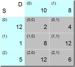
The source and destination capacities, plus the cost matrix, are put together in the transportation tableau as shown in Fig. 1. Since this is going to be implemented in code, indices here start at 0 instead of 1, so we have D₀ and D₁ for our destinations, and S₀, S₁, S₂ as sources (top row and left column, respectively). The rest of the table shows the cost matrix, with the costs for each S_i-D_j transport route. Numbers in parenthesis are the indices of the coefficients. Big numbers in the source column and destination row are capacities, and big numbers in the matrix are costs per unit.

We need to get the algorithm started by finding an initial solution. Any solution will do, as long as all source capacity is used, and all destinations receive delivery of their full capacities.

Fig. 2	Fig. 3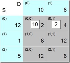
Fig. 4	Fig. 5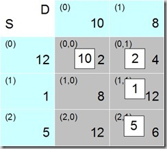

Feasible Solution

We call this a feasible solution, and the algorithm uses it as a starting point to improve in several steps until a solution is found that has minimal cost. An easy way to find such a feasible solution is to start with one cell of the cost matrix and assign it as many units as possible, and then move on to the next etc.

Starting in the example tableau with the upper left cell (0,0), we see that S₀ can deliver 12 units, and D₀ wants 10, so the maximum that can be apportioned here is 10 (Fig. 2).

That leaves the demand of D₀ completely satisfied, so we are done with column 0. Row 0 has 2 units left now, and we take these and move to column 1, which in cell (0,1) leads to a remaining source  capacity of 2, and a demand from D₁ of 8. We assign the maximum possible of 2 to this cell. The capacity of S₀ is now exhausted, and row 0 finished.

We still have excess demand from D₁, though. 2 units are being delivered to D₁ so far, of a total demand of 8, so we need to get another 6 units to D₁. Moving on to cell (1,1), we see that S₁ can deliver 1 unit, so this is assigned, and 5 more units needed for D₁. Row 1 is done, because we have used the complete capacity of S₁.

Moving to cell (2,1), we have the remaining demand of 5 units from D₁, and the capacity of 5 units from S₂, which match quite nicely. We assign the 5 units and have our feasible solution.

Initial Solution
Deliver from	Deliver to	Units	Cost per unit	Cost
S0	D0	10	2	20
S0	D1	2	4	8
S1	D1	1	12	12
S2	D1	5	6	30
			Total	70

Table 1

Fig. 5 shows the allocations in the transportation tableau, and the related cost calculations are in the table. The solution allocates all available capacity (18 units) at a total cost of 70.

This simple method to arrive at a solution is called the North-West Corner Method, because if the tableau was a map instead of being a tableau, then the starting cell would be Alaska (or Xinjiang, depending on where you are).

Dual Values

Under the hood of the transportation tableau, there is a much bigger simplex tableau, of which the transportation one is a convenient short form. In the world of the simplex algorithm, each linear program has an associated dual program that can in certain cases be used to find a solution, but that in any case can give us additional information about the original one. This is where we get the term dual values from. I am not dwelling on the mathematics, but just show how to calculate and what to do with them.

We calculate a dual u_i for each S_i, and a dual v_j for each D_j, by using the following equations for all cells in our current solution:

C_ij = u_i + v_j

 

which is obviously the same as any of

u_i = C_ij – v_j
v_j = C_ij – u_i

 

We don’t know any of the u_i, v_j yet, but are allowed to set one of them to an arbitrary value to get the calculations going. Traditionally, one would set u₀=0 to start with.

Fig. 6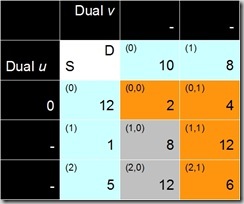

Fig. 7

In Fig. 6 we add a row and a column to the transportation tableau to hold the dual values; they are all shown as unknown, except for u₀, which is set to 0. The rest of them can now be calculated from the cost cells that are in the current solution. The rule is that the sum of each pair u_iv_j of dual values needs to be equal to the corresponding cost cell, which leads to the values in Fig. 7.

Find an Entering Cell

The dual values are now used to find a cell that is not currently in the solution and should be in there. They allow us to calculate for each of the non-solution (more correctly we ought to call them non-basis, but we won’t) cells the contribution it can make to overall cost. If for any of the cells this contribution is negative, then it is worth having the cell in the new solution. If the value is negative for more than one cell, we choose the one that can contribute most. The value we are after is the difference between the cost for each non-solution cell (i,j) and the sum of the corresponding duals, i.e.

C_ij - u_i + v_j

 

Fig. 8

Fig. 9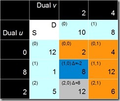

These differences have been calculated and annotated in Fig. 8. We get a value of 8 for cell (2,0), which is positive and thus not of interest. Cell (1,0), however, has –2, so we could get some cost reduction here if we get the cell into the solution (basis). 

The trick is to find a valid path from the entering cell through the current solution and back, then select one of the cells of the current solution, eliminate it, and replace it with the entering cell.

For the path-finding step we have the stepping stone algorithm, which was explained at length in a previous post. The result of applying that algorithm is shown in Fig. 10 (the dual column and row have been stripped off, because they are not needed any longer). This means that one of the cells (0,0), (0,1), or (1,1) will have to go and make room for the new cell (1,0).

Fig. 10

Fig. 11

Fig. 11 shows the capacities that were apportioned to each cell of the solution in the beginning, because this information is now needed again. The new cell (1,0) currently contributes nothing. Cell (2,1) is in the solution, but is not on the path for the new cell, so is not in danger of being eliminated.

Eliminating a Cell from the Basis/Solution

The capacities now need to be shifted between the cells on the path, so that we end up with one of them contributing nothing, so that it can be removed from the solution.

The basic idea is that whenever we add something to one of the cells, the same amount needs to be subtracted from the other cells in the same row and column, so that the totals for each row and column do not change. In terms of calculations, we go through the path, and find the minimum of every other cell. In the example tableau, this would be the minimum of (0,0) and (1,1), which is 1. We go through the path again, and subtract this value from the first cell, add it to the next, subtract from the first etc., i.e. subtract from (0,0), add to (0,1), subtract from (1,1), add to (1,0).

Fig. 12

Fig. 13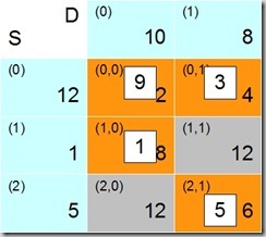

Fig. 12 shows the result of this operation. Note how the capacities assigned to each cell in the solution (plus entering cell) miraculously add up to the correct totals for each row and column, which shows us that the new solution is as feasible as the previous one.

As we did in Table 1 for the old solution, we calculate the overall cost for this new one.

New Solution
Deliver from	Deliver to	Units	Cost per unit	Cost
S0	D0	9	2	18
S0	D1	3	4	12
S1	D0	1	12	8
S2	D1	5	6	30
			Total	68

Table 2

Total cost is now 68, which is lower than what we had before, as it should be.

New Solution

Cell (1,1) does not contribute anything anymore, so can get taken out of the solution, which leads to the new solution as shown in Fig. 13. There is no guarantee that this solution is now optimal, subsequent steps may show further improvements. In order to find out, we need to take the new solution and perform the same steps again as before, starting with the calculation of the dual values.

Fig. 14

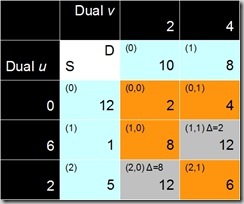
The tableau in Fig. 14 shows the result of first calculating the duals from the basis cells, and then calculating the differences between non-basis cell costs and duals. All the differences are positive (as you would expect for cell (1,1), because entering this cell would just revert to the previous solution). So there is no cell that we would want to enter into the solution and the solution that we have found is indeed the optimal one.

To be continued

The next posts will show some actual F# code to implement the steps outlined above.

Transportation Algorithm in F#, Part 2 has the F# code for all the steps of the algorithm.

Transportation Algorithm in F#, Part 3 puts those pieces together to form a working program.