F#/FsYacc: Processing the Syntax Tree in C#, Part 1

The F# PowerPack comes with the FsLex and FsYacc tools that make it quite easy to create a parser for domain-specific languages, or just to parse the contents of complex text files. A previous post had an example that took the contents of a spread sheet cell and converted it into an abstract syntax tree (AST) and also some code to walk that AST to produce a string representation that closely resembled Lisp syntax.

The parser from the example creates a syntax tree whose nodes are expressed as F# Discriminated Unions. Processing such a tree in F# is very easy and straightforward, because an AST that is built this way lends itself to be walked using recursion and pattern matching, which are obvious strengths of the programming language.

Things get a wee bit uglier when you just use F# for the lexing and parsing bit, but your main program is written in another .NET language (C# comes to mind). Discriminated unions are a speciality of F# and have no equivalent in C#, meaning that you need some strategy to deal with this situation, which is probably not a very rare one.

Discriminated Union Internals

The definition of a discriminated union on the Microsoft web site looks like this:

type type-name =
   | case-identifier1 [of type1 [ * type2 ...]
   | case-identifier2 [of type3 [ * type4 ...]
   ...

One would suspect that there must be some way to represent such a data structure in the CLR, and a bit of digging in an F# assembly shows that the underlying implementation is realised through a class hierarchy and inheritance, which after all is the CLR’s programming paradigm and is comprehensible to all languages that run on the platform.

Fig. 1

The type name as defined in the F# program, plus all the case identifiers are represented by classes. Each case identifier gets its own class that derives from a common base class, which itself corresponds to the F# discriminated union type. To keep things neatly together, all the derived classes (the case identifiers) are nested within the base class.

On the F# side, each of the case identifiers can have a type that determines what sort of data it can hold. Sometimes, a case identifier does not have a data type and only serves as a ”typed marker”, as is the case with the None case of an option type.

From the point of view of the CLR, the data associated with a case identifier become Item properties of the corresponding class. The type of the Item property is the one defined in the DU, and if the type happens to be a tuple, then each of the tuple elements becomes a separate property Item1…Itemn.

Consider the following example definition and values for a DU type:

module public Module1

type SomeUnion =
    | AWholeNumber of int
    | AString of string
    | AStringTuple of string * string
    | AStringList of string list
    | AStringArray of string array

let aWholeNumber = AWholeNumber(12)
let aString = AString("twelve")
let aStringTuple = AStringTuple("one", "two")
let aStringList = AStringList(["one";"two"])
let aStringArray = AStringArray([|"one";"two"|])

All the value bindings in this code are of type SomeUnion to the CLR (and to a C# program that wants to access them). SomeUnion corresponds to <type-name> in the class diagram above. The actual type of each value, however, is given by the constructor that was used in the F# code, i.e. the actual types are AWholeNumber, AString, AStringTuple, AStringList, or AStringArray, each of which derive from SomeUnion.

A C# program that wants to access them first needs to downcast from the type SomeUnion to the correct runtime type and can then use the Item properties to get the data:

int aWholeNumber = ((Module1.SomeUnion.AWholeNumber)Module1.aWholeNumber).Item;

string aString = ((Module1.SomeUnion.AString)Module1.aString).Item;

Tuple<string, string> aStringTuple = Tuple.Create(
    ((Module1.SomeUnion.AStringTuple)Module1.aStringTuple).Item1,
    ((Module1.SomeUnion.AStringTuple)Module1.aStringTuple).Item2);

IEnumerable<string> aStringList =
    ((Module1.SomeUnion.AStringList)Module1.aStringList).Item;

string[] aStringArray =
    ((Module1.SomeUnion.AStringArray)Module1.aStringArray).Item;

Two observations here: You can’t really use F# lists in C# code, but they can always be treated as type IEnumerable<>, which they are. In order to make this work, however, you need to add a reference to the FSharp.Core assembly to the C# project. Secondly, the way to make a C# tuple out of the F# tuple is supremely clumsy; structurally, they are the same, so there should be a more elegant way to assign one to the other^[1]. Also, in this example and in those that follow, variables are declared with their full types. In practice, one would use type inference and just declare them as var, but in the examples it is easier to see what is happening when full type names are given.

In the example above, the runtime types of all the values are known in advance, so the casting doesn’t pose any problems. When dealing with real-world F# discriminated unions, one needs to take into account that the actual type first needs to be determined in order for the casts to be successful. Three mechanisms are available:

Module1.SomeUnion.AWholeNumber aNumber = Module1.aValue as Module1.SomeUnion.AWholeNumber;
if (aNumber != null)
{
    // now we know we can cast
}

We can use the C# as keyword to try and cast; if the cast to this particular class is not successful, we try the next etc.

if (Module1.aValue.IsAWholeNumber)
{
    // now we know we can cast
}

The base class also has an Is<case-identifier> property for every derived class, in our case there is an IsAWholeNumber, IsAString, IsAStringTuple, IsAStringList, and an IsAStringArray property, so every single possibility can be checked. Internally, this uses the previous technique to try and cast to a particular type, and returns false if that cast fails.

switch (Module1.aValue.Tag)
{
    case Module1.SomeUnion.Tags.AWholeNumber:
        // cast here
        break;
    case Module1.SomeUnion.Tags.AString:
        // or cast here
        break;
    // etc.
}

Last but not least, a big switch statement on the Tag property of the base class SomeUnion will do. The value of this property is an integer that specifies the actual class being used; there is a corresponding nested struct Tags that contains one int const value with the name of each of the subclasses/case identifiers and can be used for the branches in the switch. After figuring out what the actual class is, cast the value into it, and then access the Item property, or the Itemn properties as appropriate.

Walking the AST in C#

Looking back at the original post on FsYacc, the parser created an AST with the following (recursive) structure:

type Cell =
    | FormulaCell of Expression
    | ConstantCell of Value

and Expression =
    | CellRef of Reference
    | Function of String * Expression
    | Constant of Value
    | InfixOperation of BinaryOperator
    
and BinaryOperator =
    | Plus of Expression * Expression
    | Minus of Expression * Expression
    | Times of Expression * Expression
    | Divide of Expression * Expression

and Value =
    | Float   of Double
    | Integer of Int32

and Reference =
    | SingleCellRef of String
    | RangeCellRef of String * String

Armed with the knowledge on how to access discriminated unions and their contents, the F# walker function that converts the AST into a string representation now practically rewrites itself in C#.

public static string format(Ast.Cell cell)
{
    switch (cell.Tag)
    {
        case Ast.Cell.Tags.FormulaCell:
            return format(((Ast.Cell.FormulaCell)cell).Item);
        case Ast.Cell.Tags.ConstantCell:
            return format(((Ast.Cell.ConstantCell)cell).Item);
    }

    return "<unknown cell type>";
}

public static string format(Ast.Expression expression)
{
    switch (expression.Tag)
    {
        case Ast.Expression.Tags.CellRef:
            return format(((Ast.Expression.CellRef)expression).Item);
        case Ast.Expression.Tags.Function:
            {
                var fn = (Ast.Expression.Function)expression;
                return "(" + fn.Item1 + "," + format(fn.Item2) + ")";
            }
        case Ast.Expression.Tags.Constant:
            return format(((Ast.Expression.Constant)expression).Item);
        case Ast.Expression.Tags.InfixOperation:
            return format(((Ast.Expression.InfixOperation)expression).Item);
        case Ast.Expression.Tags.ListExpression:
            {
                var sb = new System.Text.StringBuilder();

                foreach (var elem in ((Ast.Expression.ListExpression)expression).Item)
                {
                    if (sb.Length > 0)
                        sb.Append(',');
                    sb.Append(format(elem));
                }

                return sb.ToString();
            }
    }

    return "<unknown expression type>";
}

public static string format(Ast.Value value)
{
    switch (value.Tag)
    {
        case Ast.Value.Tags.Float:
            return ((Ast.Value.Float)value).Item.ToString();
        case Ast.Value.Tags.Integer:
            return ((Ast.Value.Integer)value).Item.ToString();
    }
    return "<unknown value type>";
}

public static string format(Ast.Reference reference)
{
    switch(reference.Tag)
    {
        case Ast.Reference.Tags.SingleCellRef:
            return ((Ast.Reference.SingleCellRef)reference).Item;
        case Ast.Reference.Tags.RangeCellRef:
        {
            var range = (Ast.Reference.RangeCellRef)reference;
            return "(" + range.Item1 + "," + range.Item2 + ")";
        }
    }

    return "<unknown reference type>";
}

public static string format(Ast.BinaryOperator op)
{
    switch (op.Tag)
    {
        case Ast.BinaryOperator.Tags.Plus:
            {
                var pair = (Ast.BinaryOperator.Plus)op;
                return "(+," + format(pair.Item1) + "," + format(pair.Item2) + ")";
            }
        case Ast.BinaryOperator.Tags.Minus:
            {
                var pair = (Ast.BinaryOperator.Minus)op;
                return "(-," + format(pair.Item1) + "," + format(pair.Item2) + ")";
            }
        case Ast.BinaryOperator.Tags.Times:
            {
                var pair = (Ast.BinaryOperator.Times)op;
                return "(*," + format(pair.Item1) + "," + format(pair.Item2) + ")";
            }
        case Ast.BinaryOperator.Tags.Divide:
            {
                var pair = (Ast.BinaryOperator.Divide)op;
                return "(/," + format(pair.Item1) + "," + format(pair.Item2) + ")";
            }
    }

    return "<unknown binary operator>";
}

The next installment will explore other ways to use FsYacc from a C# project, without having to look into the internals of F# datatypes.

[1] Clarification on Tuples

The remark about not being able to assign the F# tuples to C# tuples only holds in the context of discriminated unions. As for “normal” tuples, they are perfectly interoperable and the same CLR data type, so if you have a value in your F# code

module public Module1

let aTuple = ("abc", "def")

This can be used without problems in C# as

Tuple<string, string> tuple = Module1.aTuple;

Given this fact, it is an even greater pity that it doesn’t work with DUs. If the “tuple-type” cases were not implemented with a number of different Itemn properties, but with a single Item property of type Tuple<>, this could have been so much more elegant. The current implementation is probably due to the fact that the generic Tuple<> class is relatively new to C# and the CLR (this came with .NET 4), and F# tuples predate it by a few years, so interoperability wasn’t an issue at the time.

Facebook Test Users

The new test user creation facility in Facebook is quite neat and pretty straightforward. Although it is in need of some automation, especially when it comes to setting up relationships, uploading posts and pictures etc., it is way easier to handle than the old one. What you had to do until now was manually create a “normal” Facebook user, then log on as the new user and navigate to a secret web site that would then convert the account into a test account. Quite clumsy, and it needed some cleanup.

Now, what’s been bothering me: even after creating a few dozen accounts, and scripting the process to create many more, all my new users are girls. Is this some weird bias, or is it meant to keep developers in good spirit? Or is it just me?

Transportation Algorithm in F#, Part 3

After programming all the steps of the algorithm in the last post, the code in Solver.fs now puts it all together. This is a class type that can be instantiated with the problem (namely, the source and destination capacity lists, and the cost matrix) and then runs the different bits of the algorithm until an optimal solution has been found.

The only task of the constructor is to check if the input data make sense. The total source and destination capacity need to be the same, and the dimensions of the matrix need to match with the lengths of source and destination lists.

type Solver(costMatrix: int Microsoft.FSharp.Math.Matrix,
            srcCapacity: int list,
            dstCapacity: int list) =
    (*  To start with, we check if the data makes sense. If the problem
        is not balanced, or if the dimensions of the cost matrix are wrong,
        there's no point in starting the algorithm.     *)
    do if costMatrix.Dimensions <> (List.length srcCapacity, List.length dstCapacity)
        || List.sum srcCapacity <> List.sum dstCapacity then
        failwith "Invalid Data."

The most important bit of the class is the Steps member. What needs to be done here is to step through the different parts of the algorithm, check for optimality, and repeat until an optimal solution is found. A simple looping construct would suffice; I found it quite instructive, though, to be able to see the iterations with their intermediate results. Steps therefore creates a sequence that has all solutions from the initial up to the last, where the last solution in the sequence is the optimal one.

    (*  Create a sequence that gives us one intermediate solution at
        a time. The last element of the sequence is the optimal
        solution                *)
    member s.Steps =
        let rec steps sol =
            seq {
                // current solution = sequence element
                yield sol 
                // find dual values for current solution
                let duals = Dual.calc_dual_values costMatrix sol
                // for dual values, find new entering cell
                match NewBasisCell.find costMatrix duals with
                | Some(new_cell) ->
                    // use stepping stone to find path for new cell
                    let new_path = SteppingStone.find_path new_cell sol
                    // adjust values for path
                    let new_path_adjusted = NewSolution.new_path new_path
                    // from current solution and new cell's path,
                    // make new solution
                    let transformed_solution = NewSolution.transform_basis_solution sol new_path_adjusted 
                    // do it all again, with the new solution
                    yield! steps transformed_solution
                // if there's no entering cell, we're done
                | _ -> ()
            }
        // Initialisation: solution found with the North West corner method
        InitialFeasibleSolution.find_feasible_nwc srcCapacity dstCapacity |> steps

The Solution member goes directly to the end of the sequence, thus returning the optimal solution.

    (*  Go directly to last solution, which is the optimal one 
        -- See http://msdn.microsoft.com/en-us/library/system.linq.enumerable_methods.aspx
        -- for more .NET extension methods that can be used on F# sequences  *)
    member s.Solution =
        System.Linq.Enumerable.Last s.Steps

And finally, there’s a little helper method, where you can feed in a solution (e.g. one that you got out of the sequence returned by Steps) and calculate the total cost associated with that solution.

   (*  Calculate total costs for a given solution  
       -- See http://stackoverflow.com/questions/3912821/f-instance-syntax/3914236#3914236
       -- for use of __.       *)
   member __.Cost(solution: (int*int*int) list) =
       solution |> List.fold (fun acc (r, c, v) -> acc + costMatrix.[r, c] * v) 0

Running it all

Program.fs has a few lines of code that create a Solver and run it with some sample data. The code comes with two sets of data, Sample1.fs has the one used as example here, and Sample2 is a bit bigger.

let solver = Solver.Solver(costMatrix, srcCapacity, dstCapacity)

// Go through all the solutions in the sequence and
// observe the total cost going down. costs has these
// numbers in a list to print or look at in the debugger.
let costs = solver.Steps |> Seq.mapi (fun i s -> (i, solver.Cost s)) |> Seq.toList

Previous

Transportation Algorithm in F#, Part 1 explains the algorithm.

Transportation Algorithm in F#, Part 2 has the F# code for all the steps of the algorithm.

Transportation Algorithm in F#, Part 2

After having had a look at the algorithm in the last post, here is some F# code to implement it. Please not that all the source files are on CodePlex, and it may be of help to download and run that project in Visual Studio and with some strategically placed breakpoints.

File SampleData1.fs has some (surprise!) sample data. The tableau that is represented by this data is the one from the first post.

let srcCapacity = [ 12
                    1
                    5 ]

let dstCapacity = [10;8]


let costMatrix = Microsoft.FSharp.Math.Matrix.Generic.ofList
                    [   [2;4]
                        [8;12]
                        [12;6]
                        ]

Finding the Initial Solution

Sources and destinations (or rather their capacities) are represented by lists, and the cost matrix is an integer Matrix type as defined in the F# PowerPack. The very first step in the algorithm is to find a feasible solution (InitialFeasibleSolution.fs). We expect to feed in our two lists (sources and destinations) and to get another list that contains a first solution for the problem. This is of the form

[(row_number, col_number, apportioned);(row_number, col_number, apportioned);…]

For each cell in the solution, we get its co-ordinates and the capacity that has been assigned to the cell. The code looks a bit wild, but is quite simple in principle – compare the heads of the two lists, find the smaller value, remove the head from the list that has the smaller value, subtract this value from the head of the other list, and then do the same with the two resulting lists. Meanwhile, concatenate the new list with the result and return it. Oh, and carry the column and row indices with you, because we need that info. Quite simple:

let find_feasible_nwc src dst =
    let rec find_feasible src_l src_idx dst_l dst_idx =
        match src_l, dst_l with
        | h_src::t_src, h_dst::t_dst when h_src < h_dst ->
            (src_idx, dst_idx, h_src)::find_feasible 
                t_src (src_idx + 1) ((h_dst - h_src)::t_dst) dst_idx
        | h_src::t_src, h_dst::t_dst ->
            (src_idx, dst_idx, h_dst)::find_feasible 
                ((h_src - h_dst)::t_src) src_idx t_dst (dst_idx + 1)
        | _ -> []
    find_feasible src 0 dst 0

(Anyone who can come up with a way to make this tail recursive gets a special mention). There are other methods to find an initial solution, but the nice thing about the North-West Corner is that it does not require any knowledge at all about the cost matrix, so doesn’t complicate the code unnecessarily.

Dual Values

Once we have a solution, we need the dual values. The problem with this is that we cannot assume anything about the order in which we see the cells of the solution. In a small example they will look nice and tidy, but for a big tableau that has already gone through a few steps of the algorithm we must assume that they can come in any order, and not necessarily in the one that we need to be able to calculate the duals one by one. In principle, we need a topological sort first that leaves the solution cells in the order that is demanded for the calculations. But there is no way to do a topological sort nicely, without recurring to mutable state, so it’s a no-win situation. What we do here is to go through the list of cells in the solution and see how many duals we can calculate in one go. If there are any left to calculate, we do it again with the solution cells that have not contributed to the calculations yet, and so forth. In fact, this is a topological sort (compare this code to Brian’s little example that’s linked earlier, and you’ll notice it basically does the same thing), except we do it in-place, so to say. The code is in Dual.fs:

let calc_dual_values (cM: int Microsoft.FSharp.Math.Matrix) basis_solution =
    let rows, cols = cM.Dimensions
    (*  Create arrays to hold the dual values for
        sources (rows) and destinations (columns).
        To be able to express unknown quantities,
        we use arrays of option type.   *)
    let u = Array.create rows None
    let v = Array.create cols None
    (*  Here we go through all the cells of the
        current solution to see for which we
        can calculate the missing dual value.
        We can only calculate v if we have the
        corresponding u, or viceversa. 
        Any cells for which we don't have
        u or v are returned in a new list.  *)
    let rec calc sol =
        match sol with
        | [] -> [] // Not necessary, but avoids compiler warnings
        | (row, col, _) as h::t ->
            // Get the first cell
            match u.[row], v.[col] with
            // No u or v, return head and try tail
            | None, None -> h::calc t
            // u and v known. Can't really happen,
            // but again avoids compiler warnings
            | Some(ui), Some(vi) -> calc t
            // u known: calculate v, drop head, process tail
            | Some(ui), None ->
                v.[col] <- Some(cM.[row, col] - ui)
                calc t
            // v known: calculate u, drop head, process tail
            | None, Some(vi) ->
                u.[row] <- Some(cM.[row, col] - vi)
                calc t
    (*  This implements a loop that is executed until
        all u and v are known   *)
    let rec ccalc sol =
        match calc sol with // do calculations
        | [] -> ()  // all processed -> done
        | l -> ccalc l // some cells left -> try those again
    (*  Initialise an arbitrary element of one array with 0 *)
    u.[0] <- Some(0)
    (*  Start calculations *)
    ccalc basis_solution
    (*  Return two arrays with dual values.
        The arrays contain option type values; we could
        strip them off before returning them, but here we
        just let the next step of the algorithm take this
        into account and return the arrays as they are. *)
    u, v

Find Entering Cell

We now have two arrays that hold the duals for sources and destinations, respectively. In order to find the entering cell (or confirm that there isn’t any), we need to go through all non-basis (non-solution) cells, i.e. we would need to find those cells in the matrix that don’t belong to the solution. However, in order to keep the code simple, we do this for all the cells. The difference between the cost coefficient for basis cells and the duals will always be 0 (we only just calculated one from the other!), so there is no danger that we accidently choose a basis cell.

The code in NewBasisCell.fs uses the Matrix.foldi method that’s in the PowerPack and folds over all the elements of a matrix. We initiate it with a state value that has negative row and column indices, so that we know in the end if nothing has been found, and a value of 0 to compare all the dual/cost differences against. Only values <0 will be found, and of those we get the minimum, which is what we want. If we can’t have that, there’s no entering cell and the algorithm is done.

let find (cM: int Microsoft.FSharp.Math.Matrix) (u:int option array, v:int option array) =
    let (row, col, _) = 
        Microsoft.FSharp.Math.Matrix.Generic.foldi
            (fun row col ((state_row, state_col, state_value) as state) elem ->
                let value = elem - u.[row].Value - v.[col].Value
                if value < state_value then
                    (row, col, value)
                else
                    state) 
            (-1, -1, 0) cM
    if row >= 0 && col >= 0 then Some(row, col, 0) else None

If there is an entering cell, it is returned as a tuple with the row and column indices, and the capacity, so it has the same format as the elements of the current solution list, and can thus be conveniently inserted into that list. The initial capacity is set to 0 as required.

Find Path for Entering Cell

This code was already explained in the previous post about the Stepping Stone algorithm, please see there. The function in SteppingStone.fs is a bit different from what we had earlier, because we need to carry through the capacity value for the cells, so that we can use them in the next step. This wasn’t a concern with the original Stepping Stone example, but the code change is very minor. This is what the function declaration looks like with the implementation details left out:

let find_path ((targetRow, targetCol, _) as target) lstSolution =
    (* see source file *)

It takes the tuple that represents the entering cell as the first argument, and the current solution as the second, and returns a path from the entering cell through the solution. The entering cell is the first element of the returned list.

Making the New Solution

In order to go to the next solution, we need to find the minimum in the path for the entering cell (as explained in the last post), do all the additions and subtractions on the path, decide which cell to remove and remove it, and then append the cells of the old solution that were not on the path. This requires a few helper functions in NewSolution.fs.

When looking for the minimum, we only take into account every other cell on the path, starting with the second (the first one in this implementation is the entering cell). This can be done with some clever pattern matching:

let rec private find_min path = 
    match path with
    | [_;(_, _, v)] -> v
    | _::(_, _, v)::t -> min v (find_min t)
    | _ -> failwith "Unexpected data for find_min."

The function relies on there being an even number of elements in the list, and this will always be the case. If it is not, we are in trouble, and tell the user that we are. Can’t happen, though. Really.

Next, we need a function that adds/subtracts the minimum that we found from all elements on the path. Again, this only works for even numbers of elements, but we’re safe.

let new_path path =
    let m = find_min path
    let rec flatten p =
        match p with
        | (r1, c1, v1)::(r2, c2, v2)::t -> 
            (r1, c1, v1 + m)::(r2, c2, v2 - m)::flatten t
        | _ -> []
    flatten path    

We go through the path now and see which element has a capacity value of 0. In principle, there can be more than one, if the problem is degenerate. This would need special treatment, because otherwise we could end up with an endless loop in the algorithm. Keeping in mind that there is still some work to do on the fringes, which can be left for later, we just remove the first zero element that we find. The function remove_first is shown elsewhere, but here we have a little helper function that makes sure we don’t remove the very first element of the list (the entering cell) – which, in fact, can’t really happen anyway, can it?

let rec private remove_first_zero_t =
    function    | (h::t) -> h::remove_first (fun (_, _, v) -> v=0) t 
                | _ -> []

With all this in place, we can now write the function that takes the old/current solution, and the path with the entering cell, and makes a new solution out of these.

let transform_basis_solution solution new_path =
    let change_set = 
        new_path |> Seq.map (fun (r, c, _) -> (r, c)) |> Set.ofSeq
    let nonzero_new_path =
        new_path |> remove_first_zero_t
    solution 
    |> List.filter (fun (r, c, _) -> not (change_set.Contains(r, c)))
    |> List.append nonzero_new_path

We have all the bits in place now to run the algorithm, all that’s missing is some control structure that initiates it, finds out when it’s finished, and gives back the result.

To be continued

Transportation Algorithm in F#, Part 3 puts those pieces together to form a working program.

Previous

Transportation Algorithm in F#, Part 1 explains the algorithm.

Transportation Algorithm in F#, Part 1

The article on how to implement the stepping stone algorithm in F# was mainly meant to experiment with the language a bit and to show how expressive (and succinct) the code becomes when going functional, especially if there is list processing and backtracking involved. I didn’t find the overall algorithm exceptionally interesting, but it turns out that since that post back in September, many people come to this site after a search for things like “stepping stone”, “transportation algorithm code”, or occasionally “F# group by”.

It is therefore in order to expand a bit on that previous code and show a complete program, which also makes it easier to run the example and experiment a bit with it. For easier digestion we do a quick recap of the algorithm and then see what each step could look like in code.

Transportation Problem Recap

We have a number n of suppliers or sources that each have a certain amount of something that needs to be transported to a number m of destinations or sinks, with m>0, n>0, and m and n are not necessarily the same. The capacity (amount of something) for each shall be denoted by S_i for the sources, and D_j for the destinations, with i in 1..n and j in 1..n. The total capacity for all sources shall be the same as the total capacity for all destinations. This makes the algorithm easier to implement, and it is easy to create dummy sources or destinations should this condition not hold.

Transporting a unit of something from an S_i to a D_j has an associated cost C_ij. The problem at hand is now to figure out which sources should deliver to which destinations, so that the sources get rid of all their capacity, and all the destinations’ demands are satisfied. Because the total capacities for sources and destinations is the same, it is easy to see that some sort of solution must exist. But if there is more than one solution to this, we want to find the one that causes minimal cost overall.

The Initial Setup

Fig. 1

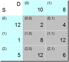
The source and destination capacities, plus the cost matrix, are put together in the transportation tableau as shown in Fig. 1. Since this is going to be implemented in code, indices here start at 0 instead of 1, so we have D₀ and D₁ for our destinations, and S₀, S₁, S₂ as sources (top row and left column, respectively). The rest of the table shows the cost matrix, with the costs for each S_i-D_j transport route. Numbers in parenthesis are the indices of the coefficients. Big numbers in the source column and destination row are capacities, and big numbers in the matrix are costs per unit.

We need to get the algorithm started by finding an initial solution. Any solution will do, as long as all source capacity is used, and all destinations receive delivery of their full capacities.

Fig. 2	Fig. 3
Fig. 4	Fig. 5

Feasible Solution

We call this a feasible solution, and the algorithm uses it as a starting point to improve in several steps until a solution is found that has minimal cost. An easy way to find such a feasible solution is to start with one cell of the cost matrix and assign it as many units as possible, and then move on to the next etc.

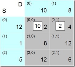
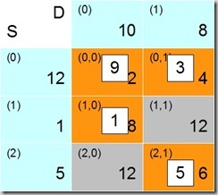
Starting in the example tableau with the upper left cell (0,0), we see that S₀ can deliver 12 units, and D₀ wants 10, so the maximum that can be apportioned here is 10 (Fig. 2).

That leaves the demand of D₀ completely satisfied, so we are done with column 0. Row 0 has 2 units left now, and we take these and move to column 1, which in cell (0,1) leads to a remaining source  capacity of 2, and a demand from D₁ of 8. We assign the maximum possible of 2 to this cell. The capacity of S₀ is now exhausted, and row 0 finished.

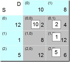
We still have excess demand from D₁, though. 2 units are being delivered to D₁ so far, of a total demand of 8, so we need to get another 6 units to D₁. Moving on to cell (1,1), we see that S₁ can deliver 1 unit, so this is assigned, and 5 more units needed for D₁. Row 1 is done, because we have used the complete capacity of S₁.

Moving to cell (2,1), we have the remaining demand of 5 units from D₁, and the capacity of 5 units from S₂, which match quite nicely. We assign the 5 units and have our feasible solution.

Initial Solution
Deliver from	Deliver to	Units	Cost per unit	Cost
S0	D0	10	2	20
S0	D1	2	4	8
S1	D1	1	12	12
S2	D1	5	6	30
			Total	70

Table 1

Fig. 5 shows the allocations in the transportation tableau, and the related cost calculations are in the table. The solution allocates all available capacity (18 units) at a total cost of 70.

This simple method to arrive at a solution is called the North-West Corner Method, because if the tableau was a map instead of being a tableau, then the starting cell would be Alaska (or Xinjiang, depending on where you are).

Dual Values

Under the hood of the transportation tableau, there is a much bigger simplex tableau, of which the transportation one is a convenient short form. In the world of the simplex algorithm, each linear program has an associated dual program that can in certain cases be used to find a solution, but that in any case can give us additional information about the original one. This is where we get the term dual values from. I am not dwelling on the mathematics, but just show how to calculate and what to do with them.

We calculate a dual u_i for each S_i, and a dual v_j for each D_j, by using the following equations for all cells in our current solution:

C_ij = u_i + v_j

 

which is obviously the same as any of

u_i = C_ij – v_j
v_j = C_ij – u_i

 

We don’t know any of the u_i, v_j yet, but are allowed to set one of them to an arbitrary value to get the calculations going. Traditionally, one would set u₀=0 to start with.

Fig. 6

Fig. 7

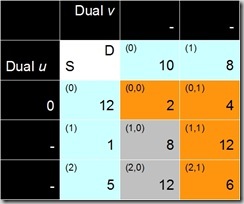
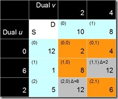
In Fig. 6 we add a row and a column to the transportation tableau to hold the dual values; they are all shown as unknown, except for u₀, which is set to 0. The rest of them can now be calculated from the cost cells that are in the current solution. The rule is that the sum of each pair u_iv_j of dual values needs to be equal to the corresponding cost cell, which leads to the values in Fig. 7.

Find an Entering Cell

The dual values are now used to find a cell that is not currently in the solution and should be in there. They allow us to calculate for each of the non-solution (more correctly we ought to call them non-basis, but we won’t) cells the contribution it can make to overall cost. If for any of the cells this contribution is negative, then it is worth having the cell in the new solution. If the value is negative for more than one cell, we choose the one that can contribute most. The value we are after is the difference between the cost for each non-solution cell (i,j) and the sum of the corresponding duals, i.e.

C_ij - u_i + v_j

 

Fig. 8

Fig. 9

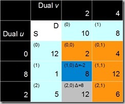
These differences have been calculated and annotated in Fig. 8. We get a value of 8 for cell (2,0), which is positive and thus not of interest. Cell (1,0), however, has –2, so we could get some cost reduction here if we get the cell into the solution (basis). 

The trick is to find a valid path from the entering cell through the current solution and back, then select one of the cells of the current solution, eliminate it, and replace it with the entering cell.

For the path-finding step we have the stepping stone algorithm, which was explained at length in a previous post. The result of applying that algorithm is shown in Fig. 10 (the dual column and row have been stripped off, because they are not needed any longer). This means that one of the cells (0,0), (0,1), or (1,1) will have to go and make room for the new cell (1,0).

Fig. 10

Fig. 11

Fig. 11 shows the capacities that were apportioned to each cell of the solution in the beginning, because this information is now needed again. The new cell (1,0) currently contributes nothing. Cell (2,1) is in the solution, but is not on the path for the new cell, so is not in danger of being eliminated.

Eliminating a Cell from the Basis/Solution

The capacities now need to be shifted between the cells on the path, so that we end up with one of them contributing nothing, so that it can be removed from the solution.

The basic idea is that whenever we add something to one of the cells, the same amount needs to be subtracted from the other cells in the same row and column, so that the totals for each row and column do not change. In terms of calculations, we go through the path, and find the minimum of every other cell. In the example tableau, this would be the minimum of (0,0) and (1,1), which is 1. We go through the path again, and subtract this value from the first cell, add it to the next, subtract from the first etc., i.e. subtract from (0,0), add to (0,1), subtract from (1,1), add to (1,0).

Fig. 12

Fig. 13

Fig. 12 shows the result of this operation. Note how the capacities assigned to each cell in the solution (plus entering cell) miraculously add up to the correct totals for each row and column, which shows us that the new solution is as feasible as the previous one.

As we did in Table 1 for the old solution, we calculate the overall cost for this new one.

New Solution
Deliver from	Deliver to	Units	Cost per unit	Cost
S0	D0	9	2	18
S0	D1	3	4	12
S1	D0	1	12	8
S2	D1	5	6	30
			Total	68

Table 2

Total cost is now 68, which is lower than what we had before, as it should be.

New Solution

Cell (1,1) does not contribute anything anymore, so can get taken out of the solution, which leads to the new solution as shown in Fig. 13. There is no guarantee that this solution is now optimal, subsequent steps may show further improvements. In order to find out, we need to take the new solution and perform the same steps again as before, starting with the calculation of the dual values.

Fig. 14

The tableau in Fig. 14 shows the result of first calculating the duals from the basis cells, and then calculating the differences between non-basis cell costs and duals. All the differences are positive (as you would expect for cell (1,1), because entering this cell would just revert to the previous solution). So there is no cell that we would want to enter into the solution and the solution that we have found is indeed the optimal one.

To be continued

The next posts will show some actual F# code to implement the steps outlined above.

Transportation Algorithm in F#, Part 2 has the F# code for all the steps of the algorithm.

Transportation Algorithm in F#, Part 3 puts those pieces together to form a working program.

MVC3 and Orchard released

Slowly coming back from hibernation, I have spent a few days trying to catch up with things that have happened in the last couple of months or so; many people have been really busy, and right now I find it difficult to catch up with everything that is going on only in the technologies I am actively using. So instead of even trying, I have opened my drawers to pull out some old code, e.g. the rest of the Transportation Algorithm that I sort of announced when writing about Stepping Stones back when. It is one of those that are quick to outline on paper, but take an awful lot of code writing. Of course, F# isn’t all that verbose, so the whole article will be up in the next few days.

There is also a new web site set up by Tomas Petricek that aims to collect little F# code snippets. It is a useful way to make single functions or one/two/three liners available to other coders, when these bits and pieces really don’t merit their own article. It also makes you feel good about yourself to give stuff away. Anyhow, I have today proudly made my first submission and will try to keep up the habit.

I also have this pet project (secret) that I once started using ASP.NET MVC 2 and recently took up again with the MVC 3 beta. So one of the highlights of the week from where I am standing is the release of MVC 3, together with some of the goodies that come with it. I love coding with Razor, it almost makes you forget you’re producing HTML. Or rather, it integrates so easily with the HTML markup that you hardly notice the clash of technologies that web development is. I guess elegant is the word.

Now you get this, and on top of it there’s a whole Content Management System that’s just a Visual Studio project template away, so to say. From what I have seen today of Orchard, integrating user and content management into your own web application will be so much more fun. I had a look into integrating bespoke web applications with CMS’es in the past; there are several dozen out there, and some are quite brilliant. Liferay is an impressive piece of work, DotNetNuke isn’t half bad either. But in the end, in order to integrate any of these big, monolithic things and their respective design philosophies within one’s own software requires to learn so many things about their internals that it is really only worth if this integration work is what you do for a living.

Imagine, however, creating an MVC 3 project that just is a CMS from the start, but where you can also have your own actions and views, and web services, and backend software and and and…

There will be a catch, or more than one, and I am planning to find out. But the thought for the day is just why didn’t I think of that?

WebSharper ¦ F# User Group

The London user group had Adam Granicz tonight talking about WebSharper in general and the upcoming version 2.0 in particular. While I like shiny new tools/toys like the next guy, I don't do much web development these days, and didn't have very high expectations. JavaScript isn't one of my favourites, and the last cool technology I remembered was the beta of ASP.NET MVC... But I must say that the presentation was way impressive. Writing web apps for the client side using a proper programming language (F#) and model seems a big step forward, and having components on the server and client communicate seamlessly using function call semantics is genius. I still have a number of doubts and questions, but there was little time and I couldn't make the social bit because I had to catch the train (which I am now sitting on, incidentally), so they have remained unanswered for now. But I understand that there is another WebSharper event here in November, and I intend to be there and report back.
--
Sent from my Android phone.